Background

A scenario is a coherent, internally consistent and plausible description of a possible future state of the world. In the sense that the term is used here, a scenario is a quantitative representation, constructed from climate model data.  Most scenarios of future climate change are based on data from General Circulation Models, or GCMs (see Understanding climate scenarios).

GCMs were originally developed and run to help climate scientists understand the Earth-atmosphere-ocean system and how it might evolve when forced with increasing atmospheric concentrations of greenhouse gases. However, it wasn’t long before the potential of these models to support work on impacts and adaptation responses was realised, and requests started to be made for climate model data. 

GCMs were never intended to be used to support work on impacts and adaptation. They were designed to model the large-scale processes of the atmosphere, rather than the small-scale processes that determine, for example, the distribution of daily rainfall.  To some extent, this imbalance has been overcome by nesting Regional Climate Models inside GCMs, to produce the fine spatial and temporal information that is desired by end users. Nevertheless, uncertainties remain, some of which can never be resolved (see Understanding climate scenarios), and so climate scenarios will always be plausible representations of future climate, rather than forecasts or predictions.  The use of climate scenarios in adaptation planning is constrained by this reality.

What scenarios are available?

Increasingly, climate modelling groups are seeking to deliver data and scenarios to impact analysts and adaptation planners. This is part of a wider initiative in ‘climate services’ – defined by the Climate Services Partnership as the ‘production, translation, transfer, and use of climate knowledge and information in climate-informed decision making and climate-smart policy and planning’ (http://www.climate-services.org/about-us/what-are-climate-services accessed 14 June 2016).

A number of modelling groups around the world have prepared climate change scenarios in different ways in an attempt to provide information that is useful to impact analysts and adaptation planners. CoastAdapt has information on what scenario information is readily available in Australia (see Accessing climate scenarios).

Projected change in mean climate.  At its simplest, a climate change scenario will depict a map of the projected change in mean climate relative to a baseline such as 1986-2005.  An example for Australian temperature and rainfall is shown in Figure 1.  Note that, whereas the temperature change is shown as a simple difference, the rainfall change is shown as a percentage. This is because rainfall amounts are highly variable across Australia, so that the simple difference fails to show the importance of a change at any particular place – a relatively small change in a dry location may have much greater significance than a larger change at a wet location.

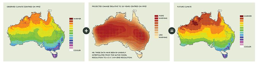
Future climate. Rather than scenarios of the change in climate, sometimes it is more useful to have a scenario of the future climate itself, complete with the characteristics of spatial and temporal variability that we observe at the present day. The Climate Change in Australia (CCiA) website calls these ‘applications ready datasets’, because they can be used in applications in exactly the same way as a dataset of the observed climate (for example to study streamflow or crop yields).  These datasets are constructed by applying the modelled change in climate to observed datasets—in the case of the CCiA by applying projected changes in monthly mean climate to 30-year average observed datasets centred on 1995 (1981-2010). This is sometimes known as the ‘delta change’ method.  An example is shown in Figure 2. For further information, see http://www.climatechangeinaustralia.gov.au/en/support-and-guidance/using-climate-projections/application-ready-data/ (accessed 14 June 2016).

Probabilistic scenarios. In an effort to overcome the difficulties caused by uncertainties around climate change projections, the UK Met Office produced a set of probabilistic scenarios, known as UKCP09.  These assign a probability to different climate change outcomes, for example, the probability that temperature will rise by more than 2 ^oC, or by between 2.5 and 3.5 ^oC. These probabilistic projections are constructed from thousands of model runs.  At the 10% probability level, only 10% of the model runs fall at or below that level; at the 90% probability level, only 10% of the climate model runs fall at or above that level. More information is available at http://ukclimateprojections.metoffice.gov.uk/21680 (accessed 14 June 2016). An example is shown in Figure 3.  Probabilistic scenarios can prove challenging to communicate to stakeholders.

Scenarios of extremes. Generally, end users such as adaptation planners are particularly interested in what will happen to extreme events in a warmer climate.  GCMs are not designed to simulate the climate at scales appropriate for studying extremes, for example, hourly rainfall data.  However, some modelling groups have been able to extract data for some variables in formats that are potentially useful. Temperature, for example, is well-simulated by GCMs, and therefore is amenable to analysis at scales that will yield useful information about extremes (see Figure 4). The Climate Change in Australia website provides a tool, the Threshold Calculator that allows the user to generate maps of changes in extreme temperatures, see http://www.climatechangeinaustralia.gov.au/en/climate-projections/explore-data/threshold-calculator/ (accessed 14 June 2016).

Data sets for further analysis. Maps and graphs of future climate change are useful for a preliminary exploration of risk, and for communicating risk. Further in-depth exploration of the impacts is likely to require datasets from GCM experiments.  With a grid resolution of a few degrees, a time step of around 20 minutes, and a run length of around 100 years, GCMs can output a vast amount of data. Modelling groups will only archive a small percentage of data, which they view as important for their own purposes, or which might be useful for end users such as adaptation planners.  Generally, modellers will carry out some ‘post processing’, so that the data can be delivered in manageable formats and file sizes. The data may be used, for example, as input to a crop-climate model, or to a hydrological model.  Figure 5 shows an example exploring future changes in runoff for Australia. The study calculates the 10^th percentile, median and 90^th percentile annual runoff from 15 GCMs. It shows clearly the uncertainties surrounding projections of rainfall in climate models, and how these uncertainties flow through into impacts analysis.  What is of great interest, however, is that whatever GCM is used, whether ‘wet’ or ‘dry’, south-west Australia is always shown to become drier in future.

How can adaptation planners use scenarios?

Scenarios of future climate change are useful in a range of situations, and it is important to choose the right scenario for the task at hand.  Ideally, they should not be used in isolation, since they are not the sole determinant of future conditions. Other factors are also changing, such as population, socio-economic status, infrastructure and markets, and all of these can be important for future planning. Wherever possible, these non-climatic factors should also be taken into account.

An important role for scenarios is in communication with stakeholders.  For this purpose, maps and graphs of future changes should be sufficient. However, there is a risk that these will appear too distant from reality, and anything that can relate the information to people’s experiences will be useful.  For example, photographs of damage caused by king tides (see The Witness King Tide project) provide a useful starting point for discussion on future sea-level rise.

Scenarios can also be useful in carrying out a preliminary or first-pass risk assessment.  Again, maps and graphs (i.e. a visual representation) may be sufficient. In this case, the uncertainty in future projections of climate change needs to be considered, and attempts made to take this into account, for example by taking some form of probabilistic approach (see Figures 3 and 5).  Where the uncertainties are considered to be high (for example with rainfall- and wind-related variables) it may be appropriate to carry out some form of sensitivity analysis. This will ask and answer questions such as:

• If gale-force winds occurred twice as often, what would this mean for the security of electricity supply, and how could we adapt?
• If we experienced drought one year in five instead of one year in ten, what would this mean for agricultural productivity, and how could we adapt? 

Sensitivity analyses are powerful tools for understanding vulnerability and exposure to risk.

A preliminary evaluation of risk may highlight areas that require further analysis (a second-pass or third-pass risk assessment), for example because the risks are deemed to be potentially unacceptably high.  In this case, it is likely that scenario data will be needed, to be used as input to impacts models. In this case, the data will generally need to be in the form of a representation of future climate, rather than the change between now and some future date (i.e. applications ready datasets, see Figure 2). It may be necessary to request these data sets from a data provider as these are not always immediately available for download.  Some experience in linking climate model data to impacts models, and in particular the effects on uncertainties, is advisable in this circumstance, and it may be necessary to hire an expert.