You are here
How to understand climate change scenarios
Scenarios are plausible climate futures, taking into account increasing atmospheric concentrations of greenhouse gases, and usually constructed from computer-based models of the Earth-Ocean-Atmosphere system. They should not be treated as predictions.
At a glance
Our climate is changing, and will continue to change because we are adding greenhouse gases to the atmosphere. To understand what the changes are likely to be, we use three-dimensional climate models, or General Circulation Models (GCMs). By changing the greenhouse gas concentrations in these GCMs, we can build scenarios of future climates. It is important to recognise that these scenarios are not predictions – they are simply ‘plausible futures’.
In using GCMs to study the future, it is important to bear in mind the following:
- Using information from a single model gridpoint in a model, or even a few gridpoints, will be misleading. GCMs were constructed to study large-scale (continental/hemispheric/global) climate, not the climate of a single local council.
- Some climate variables are better simulated by GCMs than others. That is, we can be more confident about some variables, such as sea-level rise and temperature, and less confident of others such as wind and rainfall.
- Uncertainties exist in model outputs. Some are irreducible, for example we are uncertain about how we will live in the future, will economies continue to be fossil-fuel based, or will they move strongly towards renewable energy sources? It is important to remember that model outputs provide a future that is likely for variables such as temperature and plausible for others for which there is less certainty, but not necessarily one that will occur.
- The skill and knowledge of the model data user is an important factor. The user must make choices, for example, about which greenhouse gas pathway to use. Also, climate scenarios need to be accompanied by some form of visualisation of the future community. Who will live where, what will be the economic base, where will the main infrastructure be located? For individual local councils, the best people to undertake that visualisation are likely to be council employees and residents.
Six rules for using climate models:
- Don’t rely on a single model run – use an array of model runs as the basis to identify a ‘best-guess’ scenario, or use a resource such as the Climate Change in Australia website which has gone through this exercise for you.
- Make a reasoned choice of greenhouse gas scenario: perhaps RCP8.5 to be risk averse, or RCP6.0 as the likely best guess if progress is made in the international negotiations on emissions reduction. Unfortunately a lot fewer model runs are currently available for RCP6.0.
- Always keep in mind that models only provide a scenario – a likely or plausible future – and not a prediction. The reality maybe be better, worse, or just different.
- Use model output accordingly – as a basis to explore system sensitivities and vulnerabilities, and to identify appropriate low-regrets adaptation options and their timing.
- Keep in mind the things the models can’t help you with – sudden shocks such as rapid sea-level rise and the impact of events occurring simultaneously (for example, wind storm and catchment flooding). These could happen – would your system be able to cope?
- Finally, always remember, precision does not equal accuracy!
Main text
1. What are climate models?
Projections of future climate change are carried out using climate models. These models are computer-based simulations of the Earth-ocean-atmosphere system, which use the fundamental thermodynamic equations to describe the behaviour of the system. Models come in many levels of sophistication, from the simple one-dimensional through to complex three-dimensional characterisations of the system. Even today with the very powerful computers at our disposal there are trade-offs – the more complex the model, the longer it will take to perform a model experiment. This is an important consideration when performing climate change simulations that are typically run for around 100 years out to 2100. It means that there is still a place for the more simple one- and two-dimensional models that can quickly perform long (multidecadal) runs very many times.
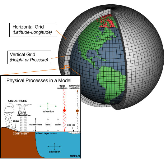
Model information for impact and adaptation studies typically comes from three-dimensional models, or General Circulation Models (GCMs). The configuration of a GCM is shown in Figure 1. These models have a three-dimensional grid and, when the model is being run, the model values (energy, pressure etc.) are calculated at the grid intersections for each time step (typically, 20 minutes). The resolution of the grid is one determinant of how long a typical 100-year model run will take. Run lengths are typically of the order of weeks to months. In order to use a GCM to study climate change, modellers will increase the concentrations of greenhouse gases in the model atmosphere, and observe the effect.
T2M1_Figure-1.jpg
2. Information from climate models: how ‘good’ is it and how should we use it?
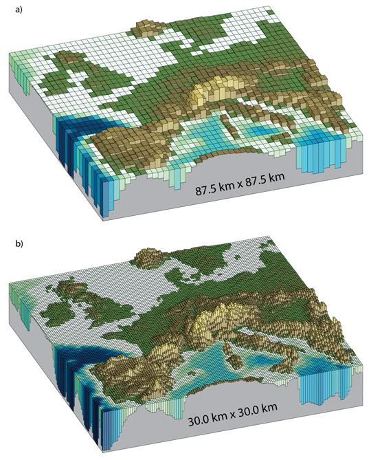
Using information from a single model gridpoint, or even a few gridpoints, will be misleading. Over time, as computers have increased in power and in size, it has become possible to increase the spatial resolution of the model grid, and the geography has therefore become more realistic (see Figure 2 and Figure 3 – note although these are for Europe, the spatial resolution of climate models over Australia has improved in the same way). Nevertheless, GCMs were not designed for impact and adaptation studies. They were designed to explore the behaviour of the atmosphere at regional to hemispheric to global scales. Modellers have never supported the extraction and analysis of model data from a single gridpoint of a model. The more model gridpoints we aggregate across, the better the model accuracy becomes.
T2M1_Figure-2.jpg
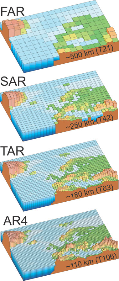
T2M1_Figure-3.jpg
Some climate variables are better simulated by GCMs than others. That is, we can be more confident about some variables. Model performance is evaluated by running the GCM with present-day concentrations of greenhouse gases and comparing the results to present-day climate. Such studies tell us that the variables of interest to impact and adaptation analysts are simulated by GCMs with different degrees of accuracy. Models are very good at simulating temperature. Their accuracy is much less for the simulation of rainfall and windstorm. However, the more we aggregate spatially across model gridpoints, and the more we average across time, the better the accuracy becomes – although local, daily rainfall is poorly simulated, regional, monthly rainfall is much better simulated by models.
This point is really well illustrated by the Climate Change in Australia website. This has a tool to construct tables showing the number of model runs (from an array of 48) that predict temperature and precipitation changes within certain bounds. You input the RCP scenario, time period and region, and the tool outputs a table. An example is shown in Table 1. As you can see, the temperature projections are reasonably consistent but the rainfall changes are all over the place: 38 percent of runs suggest drying, 18 percent suggest it will get wetter, and 23 percent show no change. A brave person might suggest the model prediction is for a drier future.
T2M1_Table1.gif
Model runs are only scenarios – plausible futures – they are not forecasts. For this reason, people usually take the output from a number of model runs (either from the same model, or from single runs of a number of different models) as a basis for constructing a scenario for impact or adaptation analysis. Possible ways of using such an array of model runs include:
- Choosing the median model estimate of future global temperature change as the ‘best guess’ of future climate conditions, and constructing a scenario from the output of that model run. The remaining models can be used to evaluate a confidence range. Thus, suppose a scenario is to be constructed from 19 model runs for the period 2070-2099. Then, the global temperature change is calculated (averaging across all model grid points for the 30 years), and the model with the median perturbation is selected as the basis for the scenario (ranked number 10). Confidence levels can be set by looking at model outliers – in an array of 19 model runs, the model with the 18th highest global temperature will represent the 90 percent confidence limit, and the model with the 2nd highest global temperature will represent the 10 percent confidence limit. This approach is used in the Climate Change in Australia (www.climatechangeinaustralia.gov.au) climate change scenarios. For more information, read Chapter 6 of the Technical Report (https://www.climatechangeinaustralia.gov.au/media/.../CCIA_Australian_cities_1.pdf).
- Making a probabilistic estimate, as was done for the UKCP09 scenarios (ukclimateprojections.metoffice.gov.uk/). This approach assigns a probability to different climate change outcomes, for example, the probability that temperature will rise by more than 3oC, or by between 3 and 3.5oC. UKCP09 constructed probabilistic projections from thousands of GCM runs. However, users have found the approach can be hard to understand and apply.
3. Choosing a greenhouse gas scenario
Climate change is simulated in GCMs by gradually increasing the atmospheric concentrations of greenhouse gases and observing the effects on the model climate. To do this, some decisions have to be made about how greenhouse gas concentrations will change in the future, and these are then translated into scenarios which are plugged into the GCM.
The best-known emissions scenarios are probably the SRES (Special Report on Emissions Scenarios (Nakicenovic and Swart 2000) scenarios, and model output based on these are still in use today for impact and adaptation studies. A drawback with these is they are ‘no-policy’ scenarios – they do not take into account the potential effects that mitigation policy might have on emissions. Increasingly they are being superseded by the RCPs (Representative Concentration Pathways) scenarios which do take into account mitigation policy (Moss et al. 2010). In practice (i.e. in terms of the effects on GCMs) it makes no difference whether a model uses an SRES or an RCP scenario. However, in the sense of attempting to model what is likely to happen in the real world in future, it is sensible to use a greenhouse gas pathway that explicitly takes into account emissions-reduction policies. Model runs being undertaken today are generally based on the RCPs.
There are four RCPs, explained in What are the RCPs? and in Figure 4. Each is designated by a number indicating how much we expect we will change the climate. The most severe is RCP8.5[1] and the least severe scenario is RCP2.6. Only in the RCP8.5 pathway do emissions of greenhouse gases continue to rise until 2100. To achieve the other three pathways, we must reduce emissions at some point and, in the 2.6 pathway, emissions start to reduce now. Only RCP2.6 and (possibly) RCP4.5 are likely to deliver a global temperature change of less than 2oC compared to pre-industrial temperatures (2oC is recognised as the threshold at which climate change becomes ‘dangerous’). Following the greenhouse gas pathway for RCP8.5 is likely to deliver warming of 4oC or more.
How should you select a greenhouse gas scenario? There are two good reasons for choosing RCP8.5. Firstly, of the current generation of model runs, it presents the ‘worst case’. That isn’t to say things couldn’t be worse, they could. But we don’t have model evidence for a case worse than RCP8.5. So it is possible to argue that, by selecting RCP8.5, you are fulfilling a duty of care by being as risk averse as possible. The second is that, globally, we are currently tracking along the RCP8.5 pathway, and therefore it can be argued that by selecting RCP8.5 you are picking the scenario that is closest to reality. Whether or not this situation is likely to continue is arguable - many would say that as mitigation policy begins to bite we will default to a lower RCP pathway such as RCP6.0 - but in terms of the evidence of present performance, RCP8.5 would be the closest.
T2M1_Figure-4.gif
4. Socio-economic futures
There is a set of socio-economic narratives of the future to accompany the RCP scenarios, known as the Shared Socio-economic Pathways or SSPs (Kriegler et al. 2012). These are global in extent, based on population, GDP and extent of globalisation. Because they are global, they may not apply at the scales relevant to coastal managers in Australia. Nevertheless, they highlight that scenarios of future climate change cannot be imposed on present-day conditions in order to understand the impacts – it is necessary to attempt to visualise the future. For individual local councils, the best people to undertake that exercise are likely to be council employees and residents. Indeed, by drawing residents into the visualisation process, councils may be able to open a constructive conversation on adaptation (Read more on Communicating climate scenarios).
5. What is uncertainty and how can it be managed?
A common argument amongst users is that model output cannot be used in adaptation planning because of the uncertainties. How true is this?
In climate models there are three main sources of uncertainty:
Scenario uncertainty: We don’t know how we will live in future, and so we don’t know which of the greenhouse gas scenarios will prove to be the one we follow, if any. Will we track along the RCP8.5 pathway, maybe 6.0 or 4.5, possibly even 2.6 or something entirely different?
Model uncertainty: We have an incomplete understanding of Earth system processes, and therefore may not characterise these properly or completely in models. Further, model characteristics such as the grid resolution mean that these processes may be incompletely represented in models. Representation of clouds is a good example – obviously clouds are important in determining where and how much rainfall occurs, and yet models are not able to reproduce clouds properly because they are smaller than the grid size of even the highest resolution GCM – they are ‘sub-grid-scale processes’.
Natural variability: The way that GCM experiments are constructed, i.e. with gradually increasing concentrations of greenhouse gases over time, means that they incorporate natural variability. Thus, if I seek to compare, say, 2090-99 to 2000-2009, I will be looking not only at the effects of greenhouse warming but also of natural variability, including such large-scale multi-year processes as El Niño events. If one of my periods contains multiple El Niño events and the other does not, that will have a substantial effect on the comparison since El Niño years are typically warmer than average globally.
People will sometimes say that they will avoid taking any adaptation action until models can provide greater certainty. This view is often expressed in parallel with a call for greater model resolution so that future scenarios can be generated with detail down to a few metres. It is important to note that having a finer-scale grid resolution does not necessarily imply reduced uncertainty. Scenario uncertainty and natural variability will still be present. Further, we may actually increase the uncertainties because the model can incorporate a new set of processes, for example cloud formation, which are accompanied by their own uncertainties. Greater precision does not imply greater accuracy.
In thinking about adaptation planning, climate model uncertainties are not the only ones. Sometimes people will talk about a cascade of uncertainties. Thus, if climate model output is used to run an impact model (for example a hydrological model to estimate the effects of climate change on river flow), then the uncertainties in the climate model are compounded by the uncertainties in the hydrological model, and so on.
Uncertainties make using climate model information tricky. You have to remember that you are dealing with a plausible, even a likely future, but one that may never eventuate. The reality may be better, or worse, it almost certainly will be different. That being the case, future scenarios are a good basis for exploring sensitivities and vulnerabilities, of a region such as a local council, or a sector such as electricity generation. Temperature and sea-level rise are well simulated by models, and therefore can form the basis for more robust planning decisions. Your judgement, together with your knowledge of the region or sector, is a key ingredient in interpreting model output as an ingredient in adaptation planning.
6. How can we make good use of model output?
As already noted, some model variables are better simulated than others and we can have greater confidence in what they are telling us. We are fortunate in CoastAdapt that sea-level rise is a reasonably robust variable with broadly stable projections between different GCMs. However, it is important to remember that there is the potential for shocks and surprises – for example sudden collapse of the West Antarctic icesheet could lead to a rapid increase in sea levels. Temperature is also well-simulated at the regional level and at timescales that are useful for adaptation (e.g. daily). This model output can be used to consider in some detail the future occurrence of heatwaves. However, variables such as rainfall and windstorm are less well simulated by models, so that we can only rely on relatively broad statements such as:
- Winter and spring rainfall is projected to decrease in southern Australia. Time in drought is projected to increase in southern Australia. Elsewhere, the signal of rainfall change is too small relative to natural variability to be able to make any firm statements.
- Tropical cyclones are projected to become less frequent with a greater proportion of high intensity storms (stronger winds and greater rainfall). A greater proportion of storms may reach south of 25oS.
The Climate Change in Australia website provides regional information on expected future climate change, at the level of four regional ‘super clusters’, eight clusters and 15 sub-clusters. As a starting point, see http://www.climatechangeinaustralia.gov.au/en/climate-projections/future-climate/regional-climate-change-explorer/super-clusters/
Six rules for using climate models:
- Don’t rely on a single model run – use an array of model runs as the basis to identify a ‘best-guess’ scenario, or use a resource such as the Climate Change in Australia website which has gone through this exercise for you.
- Make a reasoned choice of greenhouse gas scenario: perhaps RCP8.5 to be risk averse, or RCP6.0 as the best guess if progress is made in the international negotiations on emissions reduction.
- Always keep in mind that models can only provide a scenario – a plausible future – and not a prediction. The reality maybe be better, worse, or just different.
- Use model output accordingly – as a basis to explore system sensitivities and vulnerabilities, and to identify appropriate low-regrets adaptation options and their timing. (Read about the Importance of adaptation).
- Keep in mind the things the models can’t help you with – sudden shocks such as rapid sea-level rise and the impact of events occurring simultaneously (for example, wind storm and catchment flooding). These could happen – would your system be able to cope?
- Finally, always remember, precision does not equal accuracy!
[1] 8.5 indicates the additional radiative forcing caused by human activity, in watts per square metre, in 2100 relative to pre-industrial times. RCP8.5 has the highest forcing and hence the greatest impact on our climate.
Further information
Source material
CSIRO and Bureau of Meteorology, 2015: Climate Change in Australia Information for Australia’s Natural Resource Management Regions: Technical Report. Australia: CSIRO and Bureau of Meteorology. Accessed 2 March 2016. [Available at http://www.climatechangeinaustralia.gov.au/en/publications-library/technical-report/].
Cubasch, U., D. Wuebbles, D. Chen, M.C. Facchini, D. Frame, N. Mahowald, and J.-G. Winther, 2013: Introduction. In: Climate Change 2013: The Physical Science Basis. Contribution of Working Group I to the Fifth Assessment Report of the Intergovernmental Panel on Climate Change [Stocker, T.F., D. Qin, G.-K. Plattner, M. Tignor, S.K. Allen, J. Boschung, A. Nauels, Y. Xia, V. Bex and P.M. Midgley (eds.)]. Cambridge University Press, Cambridge, United Kingdom and New York, NY, USA. Accessed 2 March 2016. [Available at https://www.ipcc.ch/pdf/assessment-report/ar5/wg1/WG1AR5_Chapter01_FINAL.pdf].
Kriegler, E., B.C. O’Neill, S. Hallegatte, T. Kram, R.J. Lempert, R.H. Moss and T. Wilbanks, T. 2012). The need for and use of socio-economic scenarios for climate change analysis: a new approach based on shared socio-economic pathways. Global Environmental Change, 22, 807-822.
IPCC, 2013: Summary for Policy Makers. In: Climate Change 2013: The Physical Science Basis. Contribution of Working Group I of the Fifth Assessment Report of the Intergovernmental Panel on Climate Change [Stocker, T.F., D. Qin, G.-K. Plattner, M.Tignor, S.K. Allen, J. Boschung, A. Nauels, Y. Xia, V. Bex and P.M. Midgley (eds.)]. Cambridge University Press, Cambridge, United Kingdom and New York, NY, USA. Accessed 2 March 2016 [Available online at https://www.ipcc.ch/pdf/assessment-report/ar5/wg1/WG1AR5_SPM_FINAL.pdf].
Le Treut, H., R. Somerville, U. Cubasch, Y. Ding, C. Mauritzen, A. Mokssit, T. Peterson and M. Prather, 2007: Historical Overview of Climate Change. In: Climate Change 2007: The Physical Science Basis. Contribution of Working Group I to the Fourth Assessment Report of the Intergovernmental Panel on Climate Change [Solomon, S., D. Qin, M. Manning, Z. Chen, M. Marquis, K.B. Averyt, M. Tignor and H.L. Miller (eds.)]. Cambridge University Press, Cambridge, United Kingdom and New York, NY, USA. Accessed 2 March 2016. [Available at https://www.ipcc.ch/publications_and_data/ar4/wg1/en/ch1s1-5.html].
Moss, R., J. and Coauthors, 2010: Representative concentration pathways: a new approach to scenario development for the IPCC fifth assessment report. Nature, 463, 747-756.
Nakicenovic, N., and R. Swart, 2000: Special Report on Emissions Scenarios, Edited by Nebojsa Nakicenovic and Robert Swart, pp. 612. ISBN 0521804930. Cambridge, UK: Cambridge University Press, July 2000. Accessed 2 March 2016. [Available at http://www.ipcc.ch/ipccreports/sres/emission/index.php?idp=0].
NOAA, 2012: Top 10 Breakthroughs – The First Climate Model. National Oceanic and Atmospheric Administration, Washington. Accessed 2 December 2015. [Available online at http://celebrating200years.noaa.gov/breakthroughs/climate_model/modeling_schematic.html].